Getting Started
This section will guide you through installing and using the dtcwt library.
Installation
Installation is based on setuptools and follows the usual conventions for a Python project
$ python setup.py install
A minimal test suite is provided so that you may verify the code works on your system
$ python setup.py nosetests
This will also write test-coverage information to the cover/ directory.
Simple usage
Once installed, you are most likely to use one of four functions:
- dtcwt.dtwavexfm() – 1D DT-CWT transform.
- dtcwt.dtwaveifm() – Inverse 1D DT-CWT transform.
- dtcwt.dtwavexfm2() – 2D DT-CWT transform.
- dtcwt.dtwaveifm2() – Inverse 2D DT-CWT transform.
See Reference for full details on how to call these functions. We shall present some simple usage below.
1D transform
This example generates two 1D random walks and demonstrates reconstructing them using the forward and inverse 1D transforms. Note that dtcwt.dtwavexfm() and dtcwt.dtwaveifm() will transform columns of an input array independently:
import numpy as np
from matplotlib.pyplot import *

# Generate a 300x2 array of a random walk
vecs = np.cumsum(np.random.rand(300,2) - 0.5, 0)

# Show input
figure(1)
plot(vecs)
title('Input')

import dtcwt

# 1D transform
Yl, Yh = dtcwt.dtwavexfm(vecs)

# Inverse
vecs_recon = dtcwt.dtwaveifm(Yl, Yh)

# Show output
figure(2)
plot(vecs_recon)
title('Output')

# Show error
figure(3)
plot(vecs_recon - vecs)
title('Reconstruction error')

print('Maximum reconstruction error: {0}'.format(np.max(np.abs(vecs - vecs_recon))))

show()
2D transform
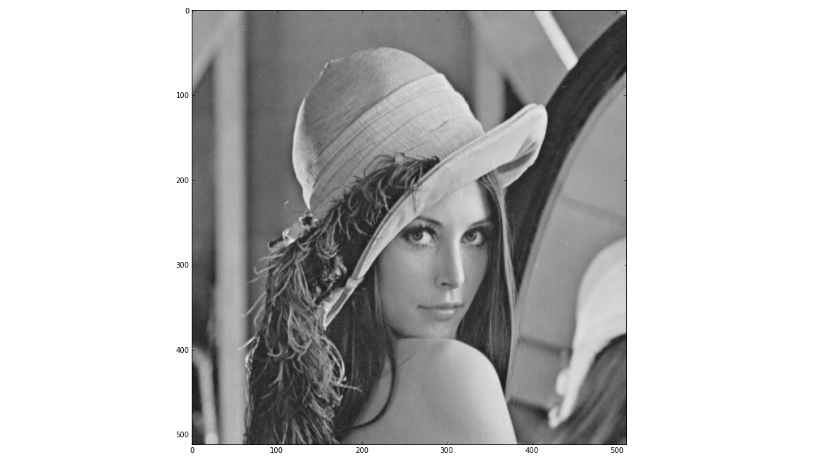
Using the pylab environment (part of matplotlib) we can perform a simple example where we transform the standard ‘Lena’ image and show the level 2 wavelet coefficients:
# Load the Lena image from the Internet into a StringIO object
from StringIO import StringIO
from urllib2 import urlopen
LENA_URL = 'http://www.ece.rice.edu/~wakin/images/lena512.pgm'
lena_file = StringIO(urlopen(LENA_URL).read())
# Parse the lena file and rescale to be in the range (0,1]
from scipy.misc import imread
lena = imread(lena_file) / 255.0
from matplotlib.pyplot import *
import numpy as np
# Show lena on the left
figure(1)
imshow(lena, cmap=cm.gray, clim=(0,1))
import dtcwt
# Compute two levels of dtcwt with the defaul wavelet family
Yh, Yl = dtcwt.dtwavexfm2(lena, 2)
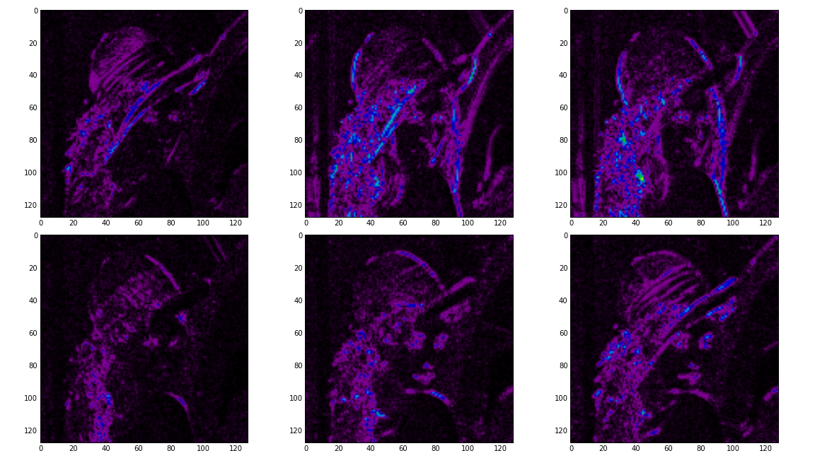
# Show the absolute images for each direction in level 2.
# Note that the 2nd level has index 1 since the 1st has index 0.
figure(2)
for slice_idx in xrange(Yl[1].shape[2]):
subplot(2, 3, slice_idx)
imshow(np.abs(Yl[1][:,:,slice_idx]), cmap=cm.spectral, clim=(0, 1))
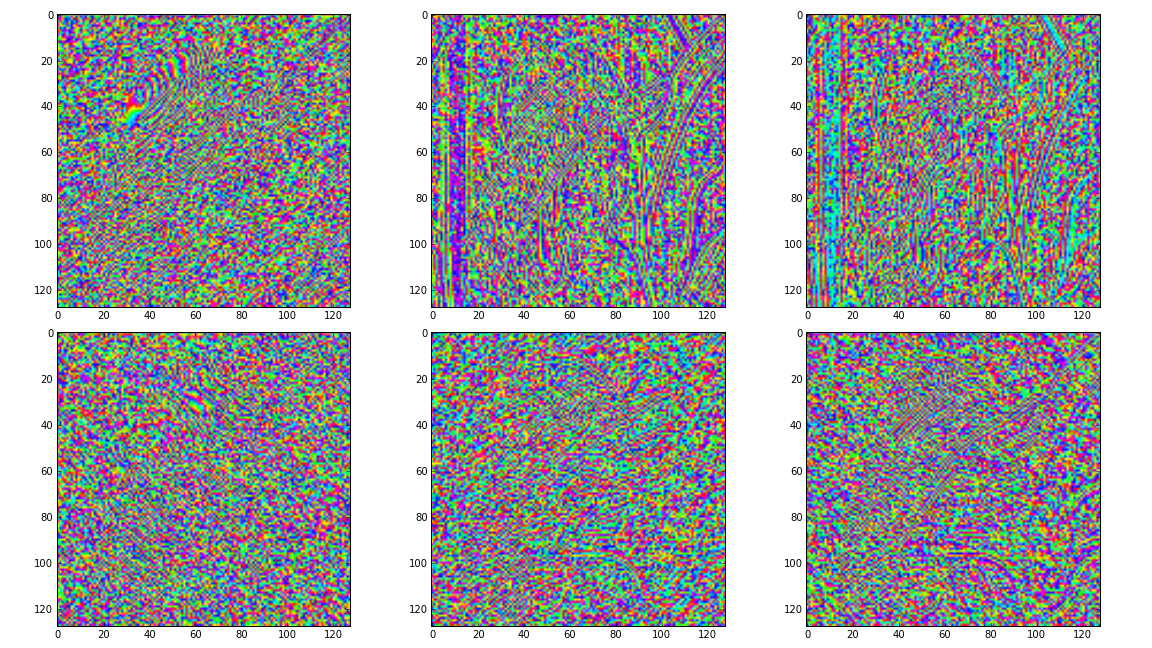
# Show the phase images for each direction in level 2.
figure(3)
for slice_idx in xrange(Yl[1].shape[2]):
subplot(2, 3, slice_idx)
imshow(np.angle(Yl[1][:,:,slice_idx]), cmap=cm.hsv, clim=(-np.pi, np.pi))
show()
If the library is correctly installed and you also have matplotlib installed, you should see these three figures: